Guitar Pitch Shifter

3. Algorithm

3.1 What needs to be achieved
3.2 Superposition of frames
3.3 Phase vocoder: 3.3.1 Overview; 3.3.2 Analysis; 3.3.3 Processing; 3.3.4 Synthesis
3.4 Resampling

3. Algorithm

We will now look at the algorithm we need to implement from a mathematical point of view.

3.1 What needs to be achieved

So now we know we first have to change the signal duration without changing the pitch. The scaling factor is defined as the factor used to stretch or compress the spectrum in order to adjust the frequencies such that the pitch is shifted. Once this is done, we will perform resampling to return to the initial duration with a shift in the pitch.

For instance, if we want to shift the pitch up by one semitone, we need a scaling factor of 2^(1/12) which equals to 1.0594. This means we first need to stretch the signal without changing the pitch such that the duration is now multiplied by 1.0594. Once this is done, we need to play the signal 1.0594 times faster.

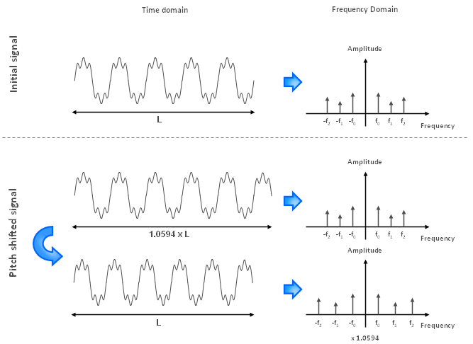
Figure 3.1: How to shift the pitch up by one semitone

On the other hand, if we want to shift the pitch down by one semitone, we need a scaling factor of 2^(-1/12) which equals to 0.9439. This means we first need to compress the signal without changing the pitch such that the duration is now multiplied by 0.9439. Once this is done, we need to play the signal slower at 0.9439 times the initial speed.

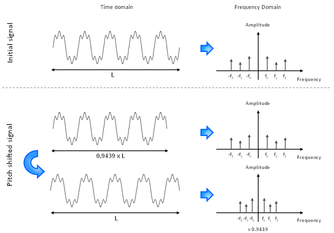
Figure 3.2: How to shift the pitch down by one semitone

3.2 Superposition of frames

We will split our signals in many small frames. These frames are taken from the initial signal such that they overlap each other by 75%. These frames will then be spaced differently in order to stretch or compress in time the output signal.

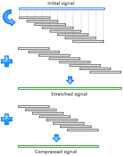
Figure 3.3: Stretching and compressing the signal frame by frame

But now we have another problem. When we space the frames differently, this creates discontinuities. This is shown in the next figure (space between frames is initially of length x and becomes of length y).

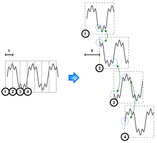
Figure 3.4: Signal discontinuities when stretching or compressing in time

This will produce glitches and will be perceived by the human ear. We need to do something to make sure there is no discontinuity. That's why we need a phase vocoder.

3.3 Phase vocoder

3.3.1 Overview

The next figure shows how the phase vocoder algorithm works. It consists of 3 stages: analysis, processing and synthesis. I will assume you are familiar with Fast Fourier Transform (FFT), Inverse Fast Fourier Transform (IFFT) and complex numbers. I will have to go through some unpleasant maths in the next subsections. I wish I could avoid this but we really need to go through these equations to understand what the algorithm does.

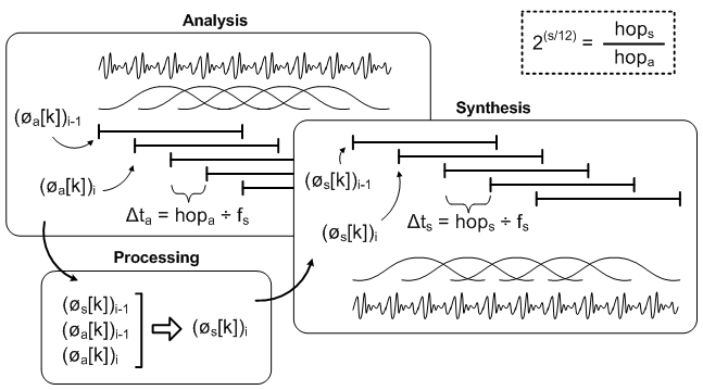
Figure 3.5: Phase vocoder overview

3.3.2 Analysis

Windowing refers to taking a small frame out of a large signal (you are only looking at your signal through a small window of time). The windowing process alters the spectrum of the signal and this effect should be minimized. In order to reduce the effect of windowing on the signal frequency representation, a Hanning window of size N is used. Why is this? Well multiplying a rectangular window with your signal in the time-domain is equivalent to performing a convolution in the frequency domain. A rectangular window has more energy in the side lobes while a Hanning window focuses most of its energy near DC. This looks more like an impulse which would lead to a perfect reconstruction of the signal.

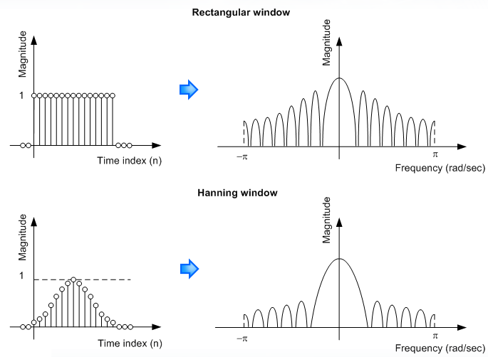
Figure 3.6: Windowing

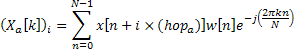
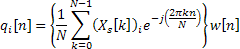
The frame made of N samples is then transformed with a Fast Fourier Transform (FFT) as shown in equation 3.1.

Equation 3.1: Analysis stage equation

In the previous equation, is the sample signal, represents the Hanning window and represents the discrete spectrum of the frame . To increase the resolution of the spectrum, the windows are overlapped with a factor of 75%. The number of samples between two successive windows is referred to as the hop size () and is equal to for an overlap of 75%.

3.3.3 Processing

Applying a FFT of length N results into N frequency bins starting from 0 up to with an interval of where is the sampling rate frequency. A signal with a frequency that falls between two bins will be smeared and its energy will be spread over the nearby bins. The phase information is used to improve the accuracy of the frequency estimation of each bin. Figure 3.7 shows two sine waves with slightly different frequencies. These frames are divided into frames of N samples. Windows do not overlap in this case to make the explanation simpler. The first sine wave has a frequency of and thus falls exactly on the first bin frequency. The second wave has a frequency slightly greater than the first bin frequency. It is not centered at the first bin although its energy lies mostly in this bin.

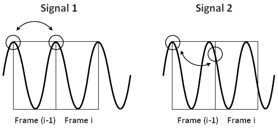
Figure 3.7: Sine waves with different frequencies and phase difference

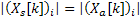
The phase information of the two successive frames is of significant interest. For the first signal, there is no phase difference between the two frames. However, for the second signal, the phase of the first bin is greater than zero. This implies that the signal component corresponding to this bin is higher than the bin frequency. The phase difference between the two frames is referred to as the phase shift . For all variables in this text, k and i stand for bin index and frame index respectively. The phase shift can be used to determine the true frequency associated with a bin. However, the phase information provided by the FFT is wrapped, which implies that lies between –pi and pi. Without wrapping, the true frequency can be easily obtained from the phase shift and the time interval between two frames as shown in equation 3.2. The time interval is the hop size divided by the sampling rate frequency .

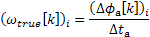
Equation 3.2: True frequency when the phase shift is unwrapped

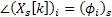
The matter is more complex since the phases are wrapped. In this case, the frequency deviation from the bin is first calculated and is then wrapped. This amount is added to the bin frequency to obtain the true frequency of the component within the frame. Equations 3.3, 3.4 and 3.5 illustrate this procedure. The variables and stand for the phase of the previous frame and the current frame respectively. Also, stands for the bin frequency, stands for the frequency deviation and 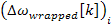stands for the wrapped frequency deviation.

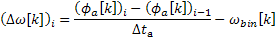
Equation 3.3: Frequency deviation

Equation 3.4: Wrapped frequency deviation

Equation 3.5: True frequency

The new phase of each bin can then be calculated by adding the phase shift required to avoid discontinuities. This is done by multiplying the true frequency with the time interval of the synthesis stage as shown in equation 3.6.

Equation 3.6: Phase adjustment for the synthesis stage

The phase of the previous frame for synthesis is known since it was already calculated as the algorithm is recursive. The new spectrum is then obtained as shown in equation 3.7.

Equation 3.7: Amplitude and phase of the spectrum of the synthesis stage

3.3.4 Synthesis

So now we managed to adjust the phase in the frequency domain for our current frame. We need to come back to the time domain. The inverse discrete Fourier transform (IDFT) is performed on each frame spectrum. The result is then windowed with a Hanning window to obtain . Windowing is used this time to smooth the signal. This process is shown in equation 3.8.

Equation 3.8: Synthesis stage equation

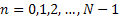
Each frame is then overlap-added as shown in equation 3.9. The variable stands for the number of frame and represents the unit step function.

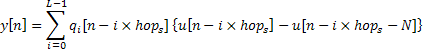
Equation 3.9: Overlap-add of the synthesis frames

Sorry about that, it was really painful I know. The good news is that we’re done with most of the maths now.

3.4 Resampling

Hey, good news! We have our signal that is now either stretched or compressed in time and the pitch is not changed. Now we need to resample our signal to get back to the initial duration and shift the pitch. Suppose I have a given sampling rate and I want to double the frequencies. The easiest thing to do is to pick only one sample out of two and to output the result.

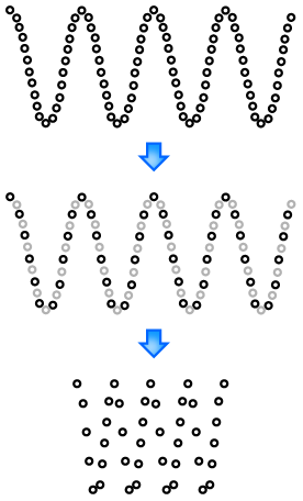
Figure 3.8: Resampling at twice the previous rate

Now this is easy because when we double the frequency we deal with a scaling factor that is an integer. If the scaling factor is not an integer (for instance 1.0594 when we shift the pitch up by one semitone), then we cannot use the same technique. We will use instead linear interpolation to approximate the sample that should lie at this location. Linear interpolating also behaves like a low-pass filter and thus removes most of the possible aliasing when we downsample. The next figure shows an example with a scaling factor of 1.2.

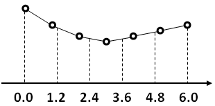
Figure 3.9: Linear interpolation

Okay, we are done with the algorithm!

Previous: Pitch shifting

Next: Hardware